2.5. Appendix: Python code
import numpy as np
import matplotlib.pyplot as plt

plt.style.use(['seaborn-ticks', 'seaborn-talk'])
n_energy_levels= 10
reducedTemperatures=[0.5, 1, 2, 3]
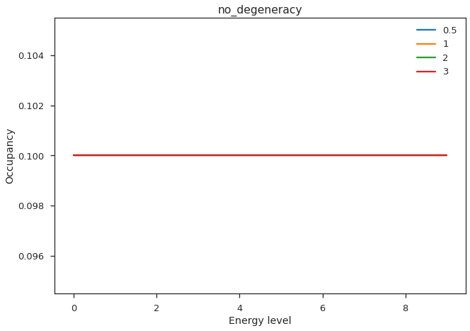
def calculateStateOccupancy(T, i):
# No degeneracy
#MODIFY HERE
return 1
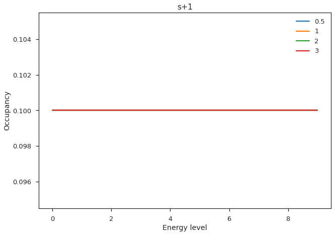
def calculateStateOccupancy_s1(T, i):
# Degeneracy s+1
# MODIFY HERE
return 1
def calculateStateOccupancy_s5(T, i):
# Degeneracy s+5
# MODIFY HERE
return 1
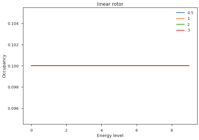
def calculateStateOccupancy_rotor(T, i):
# Linear Rotor
# MODIFY HERE
return 1
functions ={
"no_degeneracy": calculateStateOccupancy,
"s+1": calculateStateOccupancy_s1,
"s+5": calculateStateOccupancy_s5,
"linear rotor": calculateStateOccupancy_rotor
}
for f in functions.keys():
fig, ax =plt.subplots(1)
ax.set_title(f)
ax.set_xlabel("Energy level")
ax.set_ylabel("Occupancy")
calculateOccupancy=functions[f]
for reducedTemperature in reducedTemperatures:
distribution = [] # For each state there is one entry
partition_function=np.float64(0.0)
for i in range(n_energy_levels):
stateOccupancy=calculateOccupancy(reducedTemperature, i)
distribution.append(1.0) # MODIFY HERE
partition_function+=1.0 # MODIFY HERE
ax.plot(distribution/partition_function, label=reducedTemperature)
ax.legend()
plt.show()

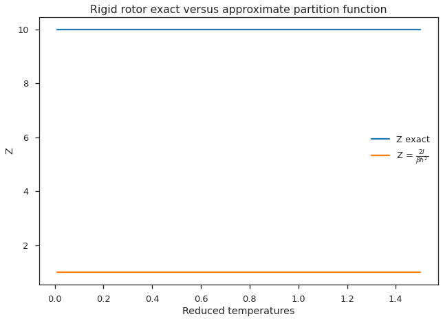
2.6. Comparison linear rotor approximate versus analytical Z
fig, ax =plt.subplots(1)
ax.set_title('Rigid rotor exact versus approximate partition function')
ax.set_xlabel("Reduced temperatures")
ax.set_ylabel("Z")

n_energy_levels = 10
reducedTemperatures=[0.01, 0.1, 0.25, 0.5, 0.75, 1, 1.5 ]

list_of_exact_Z = []
list_of_approx_Z = []

#iterate over reduced temperatures and add Z value for that temperature to list
for reducedTemperature in reducedTemperatures:

    Z=np.float64(0)

    # exact partition function
    for i in range(n_energy_levels):
        stateOccupancy=1 # MODFIY HERE
        Z+=1 # MODFIY HERE
    list_of_exact_Z .append(Z)

    # approximate partition function
    approx_Z =1 # MODFIY HERE
    list_of_approx_Z.append(approx_Z)

ax.plot(reducedTemperatures,list_of_exact_Z, label="Z exact" )
ax.plot(reducedTemperatures,list_of_approx_Z, label =  r'Z = $\frac{2 I}{\beta \hbar^2}$')

ax.legend()
plt.show()