3.2. Exercises
For the second exercise we need to install a package and create a virtual environment for it.
For JupyerHub, connect using this link, open the terminal and type the following commands:
python3 -m venv ~/my_venvs/mdmc
source ~/my_venvs/mdmc/bin/activate
pip install --upgrade pip
pip install numpy matplotlib ipykernel py3Dmol
python3 -m ipykernel  install --user --name=mdmc
While this completes (ca. 5 minutes) you can already start with the first exercise.
3.2.1. Monte Carlo and Statistical Mechanics
Show that based on the form of the Hamiltonian:
\[ \begin{aligned} \mathrm{H} = \mathrm{T}(\mathbf{p}) + \mathrm{V}(\mathbf{q}), \end{aligned} \]the partition function can be divided into a kinetic and potential part, and for an ensemble average of an observable \(O(\mathbf{q})\) that depends on \(\mathbf{q}\) only, one has:
\[\begin{split} \begin{aligned} \left<O(\mathbf{q})\right> &= \frac{\int_\Gamma O(\Gamma)e^{-\beta E(\Gamma)} \mathrm{d}\Gamma}{\int_\Gamma e^{-\beta E(\Gamma)} \mathrm{d}\Gamma} \\ &= \frac{\int O(\mathbf{q})e^{-\beta V(\mathbf{q})} \mathrm{d}\mathbf{q}}{\int e^{-\beta V(\mathbf{q})} \mathrm{d}\mathbf{q}}, \end{aligned} \end{split}\]which is the equation you have encountered in the section on detailed balance.
Bonus: In the Metropolis scheme, why is it important that \(P^\prime\) be a symmetric matrix?
3.2.2. The Photon Gas
These exercises can be solved with Practical: Photon gas. Note that again we use reduced units setting \(w_j\) and \(\hbar\) to 1.
How can this scheme retain detailed balance when \(n_j = 0\)? Note that \(n_j\) cannot be negative.
Make modifications in the code, right after the commented section ‘
MODIFICATION\(\cdots\)END MODIFICATION’. Include your entire code within your report and comment upon the part that you wrote.Using your code, plot the photon-distribution (average occupation number as a function of \(\beta\epsilon \in [0.1, 2]\)). Assume that the initial \(n_j = 1\) and \(\epsilon_j = \epsilon\) and recalculate with the same \(\beta\epsilon\) values using the analytical solution:
\[ \begin{aligned} \left<N\right> = \frac{1}{e^{\beta\epsilon}-1}. \end{aligned} \]Plot your calculated values versus those from the analytical solution and include your curve in your report.
Bonus: Modify the program in such a way that the averages are updated only after an accepted trial move. Why does ignoring rejected moves lead to erroneous results? Starting from \(P_{acc} ( o \rightarrow n)\), define \(P'(o \rightarrow o)\) (i.e the probability that you stay in the old configuration). Recall that the transition probability \(P'\) is normalised.
Bonus: At which values of \(\beta\) does the error you obtain when ignoring rejected moves become more pronounced and why?
3.2.3. Sampling Configurational Space
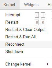
These exercises can be solved with Appendix: Configurational sampling python program. You need to select the appropriate kernel installed according to the instructions above. Perform the steps described at the top of the page and you can select the mdmc kernel for this exercise. (Note that in the Jupyter Hub interface the menu bar might look a little different).
Perform a simulation at \(T = 2.0\) and \(\rho \in 0.05, 0.2, 0.5, 1\) for 10000 steps with maximum displacement of 0.1 by executing all the cells until but not including the Visualization of results block. What do you observe? Check the energies that are printed for the steps. It is not necessary to plot the energies.
Is it justified to assume that the Lennard Jones potential can be used to describe the interaction between the particles for all values of \(\rho\)?
The program produces a sequence of snapshots of the state of the system as xyz file. You can visualise them directly in the notebook. Explain the behaviour of the system for frame 0, 1000, 5000 and 9000 for \(\rho\) 0.4
Instead of performing a trial move in which only one particle is displaced, one can do a trial move in which all particles are displaced. What do you expect will happen to the maximum displacements of these moves for a fixed acceptance rate of all displacements (for example 50%)?
Bonus Describe the changes in the code to sample from the isothermic-isobaric ensemble (NpT) instead of the microcanonical ensemble (NVT)? See end of Appendix: Configurational sampling python program.
Bonus If you set the density of particles to 10 the program will print
RuntimeWarning: overflow encountered in expand the energies will be very large. Can you still trust those energies? Explain why or why not.