3.3. Practical: Photon gas
import random as r
import math as m
import matplotlib.pyplot as plt
import numpy as np

from ipywidgets import interact, interactive, fixed, interact_manual
import ipywidgets as widgets

# Random Seed
r.seed(42)
numberOfIterations = 1000
beta = 1.0


def calculateOccupancy(beta=1.0):

    trialnj = 1
    currentnj = 1
    njsum = 0
    numStatesVisited = 0
    estimatedOccupancy=0

    """  Modification
    Metropolis algorithm implementation to calculate <n_j>
    Tasks:
    1) Loop from int i = 0 to numberOfiterations
    2) Call random(0, 1) to perform a trial move to randomly increase
        or decrease trialnj by 1.
        Hint: use trialnj = currentnj + 1;
    3) Test if trialnj < 0, if it is, force it to be 0
    4) Accept the trial move with probability defined in section 3.1.4.1
        Note: Accepting the trial move means updating current sample (currentnj)
        with the new move (trialnj);
    5) sum currentnj and increase numStatesVisited by 1

    *** END MODIFICATION ***
    """

    #estimatedOccupancy = njsum/numStatesVisited

    return estimatedOccupancy

# perform a single calculation
estimatedOccupancy = calculateOccupancy(beta=beta)
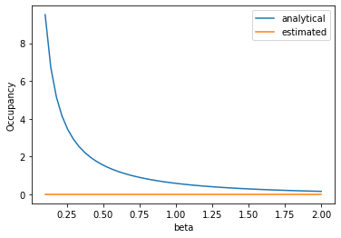
x=np.linspace(0.1,2)
analytical_y= 1/(np.exp(x)-1)
estimated_y=[calculateOccupancy(beta=b) for b in x]
fig, ax = plt.subplots(1)
ax.plot(x,analytical_y, label='analytical')
ax.plot(x,estimated_y, label='estimated')

ax.set_xlabel("beta")
ax.set_ylabel('Occupancy')
ax.legend()
plt.show()